Topics

• Calculus (50%)
  • Single Variable
  • Multivariable
  • Differential Equations

“Algebra” (25%)

• Linear Algebra
• Abstract Algebra
• Number Theory

Mixed Topics (25%)

• Real Analysis
• Logic / Set Theory
• Discrete Mathematics
• Point-Set Topology
• Complex Analysis
• Combinatorics
• Probability
  

References

Garrity, All the Mathematics You Missed (But Need to Know for Graduate School)

Good high-level overview of undergrad topics.

The Princeton Review, Cracking the Math GRE Subject Test

“Calculus: The Greatest Hits”, good breadth.

Shallow treatment of Algebra, Real Analysis, Topology, Number Theory.

Five Official Practice Exams (with Solutions)

• GR 1268
• GR 0568
• GR 9367
• GR 8767
• GR 9768

All old and significantly easier than exams in recent years.

Aim for 90th percentile in $< 2$ hours.

General Tips

Math-Specific Tips

• Focus on lower div
• For Calculus, focus on speed: median $\leq 1$ minute
• Drill a lot of problems
  • Seriously, a lot.
  • Seriously.
• Should memorize formulas and definitions
  • No time to rederive!
• Save actual exams as diagnostic tools

Study Tips

• Start early
  • Steady practice paced over 3-9 months is 100x more effective than 1 month of cramming
• Speed is important
• Spaced repetition, e.g. Anki
• Replicate exam conditions
• Build mental stamina
  • i.e. 2-3 hours of uninterrupted problem solving
• Self care!!
  • Sleep
  • Eat right

Single Variable Calculus

Differential

• Computing limits
• Showing continuity
• Computing derivatives
• Rolle’s Theorem
• Mean Value Theorem
• Extreme Value Theorem
• Implicit Differentiation
• Related Rates
• Optimization
• Computing Taylor expansions
• Computing linear approximations

Integral

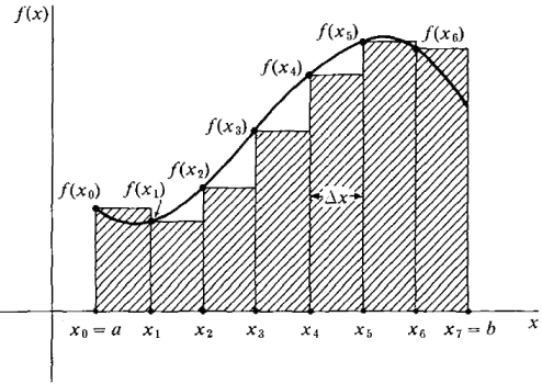
• Riemann sum definition of the integral
• The fundamental theorem of Calculus (both forms)
• Computing antiderivatives
  • $u\dash$substitutions
  • Partial fraction decomposition
  • Trigonometric Substitution
  • Integration by parts
  • Specific integrands
• Computing definite integrals
• Solids of revolution
• Series (see real analysis section)

Computing Limits

• Tools for finding $\lim_{x\to a} f(x)$, in order of difficulty:
  • Plug in: equal to $f(a)$ if $f \in C^0(N_\varepsilon(a))$
  • Algebraic Manipulation
  • L’Hopital’s Rule (only for indeterminate forms $\frac 0 0, \frac \infty \infty$)
    • For $\lim f(x)^{g(x)} = 1^\infty, \infty^0, 0^0$, let $L = \lim f^g \implies \ln L = \lim g \ln f$
  • Squeeze theorem
  • Take Taylor expansion at $a$
  • Monotonic + bounded (for sequences)

Use Simple Techniques

When possible, of course.

The Fundamental Theorems of Calculus

First form is usually skimmed over, but very important!

FTC Alternative Forms

Commuting $D$ and $I$

Commuting a derivative with an integral

(Derived from chain rule)

Applications of Integrals

• Solids of Revolution
  • Disks: $A = \int \pi r(t)^2 ~dt$
  • Cylinders: $A = \int 2\pi r(t)h(t) ~dt$
• Arc Lengths
  • $ds = \sqrt{dx^2 + dy^2},\qquad L = \int ~ds$

Series

There are 6 major tests at our disposal:

• Comparison Test
  • $a_n < b_n \and \sum b_n < \infty \implies \sum a_n < \infty$
  • $b_n < a_n \and \sum b_n = \infty \implies \sum a_n = \infty$
  • You should know some examples of series that converge and diverge to compare to.
• Ratio Test
  
  $$R =\lim_{n\to\infty} \abs{\frac{a_{n+1}}{a_n}}$$
  • $R < 1$: absolutely convergent
  • $R > 1$: divergent
  • $R = 1$: inconclusive

More Series

• Root Test
  
  $$R = \limsup_{n \to \infty} \sqrt[n]{\abs{a_n}}$$
  • $R < 1$: convergent
  • $R > 1$: divergent
  • $R = 1$: inconclusive
• Integral Test
  
  $$f(n) = a_n \implies \sum a_n < \infty \iff \int_1^\infty f(x) dx < \infty$$

More Series

• Limit Test
  
  $$\lim_{n\to\infty}\frac{a_n}{b_n} = L < \infty \implies \sum a_n < \infty \iff \sum b_n < \infty$$
• Alternating Series Test
  
  $$a_n \downarrow 0 \implies \sum (-1)^n a_n < \infty$$

Advanced Series

• Cauchy Criteria:
  • Let $s_k = \sum_{i=1}^k a_i$ be the $k\dash$th partial sum, then
    
    $$\sum a_i \text{ converges } \iff \theset{s_k} \text{ is a Cauchy sequence},$$
• Weierstrass $M$ Test:
  
  $$\sum_{n=1}^\infty \abs{\norm{f_n}_\infty} < \infty \implies \\ \exists f\in C^0 \suchthat \sum_{n=1}^\infty f_n \rightrightarrows f$$
  • i.e. define $M_k = \sup\theset{f_k(x)}$ and require that $\sum \abs{M_k} < \infty$
  • “Absolute convergence in the sup norms implies uniform convergence”

Multivariable Calculus

General Concepts

• Vectors, div, grad, curl
• Equations of lines, planes, parameterized curves
  • And finding intersections
• Multivariable Taylor series
  • Computing linear approximations
• Multivariable optimization
  • Lagrange Multipliers
• Arc lengths of curves
• Line/surface/flux integrals
• Green’s Theorem
• The divergence theorem
• Stoke’s Theorem

Geometry in $\RR^3$

Lines

Planes

Distances to lines/planes: project onto orthogonal complement.

Tangent Planes/Linear Approximations

Let $S \subseteq \RR^3$ be a surface. Generally need a point $\vector{p} \in S$ and a normal $\vector{n}$.

Key Insight: The gradient of a function is normal to its level sets.

• $\nabla f$ is a vector that is normal to the zero level set.
• So just write the equation for a tangent plane $\inner{\vector n}{\vector x - \vector p_0}$.

Tangent Planes/Linear Approximations

• Let $f(x, y, z) = g(x,y) - z$, then
  

  $$\vector p \in S \iff \vector p \in \theset{[x,y,z] \in \RR^3 \mid f(x,y, z) = 0}.\\$$

• Then $\nabla f$ is normal to level sets, compute $\nabla f = [\dd{}{x}g, \dd{}{y}g, -1]$

• Proceed as in previous case.

Optimization

Single variable: solve $\dd{}{x} f(x) = 0$ to find critical points $c_i$ then check min/max by computing $\dd{^2}{x^2}f(c_i)$.

Multivariable: solve $\nabla f(\vector x) = 0$ for critical points $\vector c_i$, then check min/max by computing the determinant of the Hessian:

Optimization

Lagrange Multipliers:

• Generally a system of nonlinear equations
  • But there are a few common tricks to help solve.

Multivariable Chain Rule

Multivariable Chain Rule

To get any one derivative, sum over all possible paths to it:

Subscripts denote variables held constant while differentiating.

Linear Approximation

Just use Taylor expansions.

Single variable case:

Multivariable case:

Linear Algebra

Big Theorems

• Rank Nullity:
  

  $$\abs{\ker(A)} + \abs{\im(A)} = \abs{\mathrm{domain}(A)}$$

• Fundamental Subspace Theorems
  

  $$\im(A) \perp \ker(A^T), \qquad \ker(A) \perp \im (A^T)$$

• Compute

  • Determinant, trace, inverse, subspaces, eigenvalues, etc
  • Know properties too!

• Definitions

  • Vector space, subspace, singular, consistent system, etc

Fundamental Spaces

• Finding bases for various spaces of $A$:

  • $\mathrm{rowspace} A/ \im A^T \subseteq \RR^n$

    • Reduce to RREF, and take nonzero rows of $\mathrm{RREF}(A)$.

  • $\mathrm{colspace} A / \im A \subseteq \RR^m$:

    • Reduce to RREF, and take columns with pivots from original $A$.

Fundamental Spaces

• $\mathrm{nullspace}(A) / \ker A$:

  • Reduce to RREF, zero rows are free variables, convert back to equations and pull free variables out as scalar multipliers.

• Eigenspace:

  • Recall the equation:
    
    $$\lambda \in \spec(A) \iff \exists \vector v_\lambda \suchthat A\vector v_\lambda = \lambda \vector v_\lambda$$
  • For each $\lambda \in \spec(A)$, compute $\ker (\lambda I - A)$

Big List of Equivalent Properties

Let $A$ be an $n\times n$ matrix representing a linear map $L: V \to W$

TFAE:

• $A$ is invertible and has a unique inverse $A^{-1}$
• $A^T$ is invertible
• $\det(A) \neq 0$
• The linear system $A\vector{x} = \vector{b}$ has a unique solution for every $b\ \in \RR^m$
• The homogeneous system $A\vector{x} = 0$ has only the trivial solution $\vector{x} = 0$
• $\rank(A) = \dim(W) = n$
  • i.e. $A$ is full rank
• $\mathrm{nullity}(A) \definedas \dim(\mathrm{nullspace}(A)) = \dim(\ker L) = 0$

Big List of Equivalent Properties

• $A = \prod_{i=1}^k E_i$ for some finite $k$, where each $E_i$ is an elementary matrix.
• $A$ is row-equivalent to the identity matrix $I_n$
• $A$ has exactly $n$ pivots
• The columns of $A$ are a basis for $W \cong \RR^n$
  • i.e. $\mathrm{colspace}(A) = \RR^n$
• The rows of $A$ are a basis for $V \cong \RR^n$
  • i.e. $\mathrm{rowspace}~(A) = \RR^n$
• $\left(\mathrm{colspace}~(A)\right)^\perp = \left(\mathrm{rowspace}~(A^T)\right)^\perp = \theset{\vector 0}$
• Zero is not an eigenvalue of $A$.
• $A$ has $n$ linearly independent eigenvectors

Various Other Topics

• Quadratic forms
• Projection operators
• Least Squares
• Diagonalizability, similarity
• Canonical forms
• Decompositions ($QR, VDV^{-1}, SVD,$ etc)

Ordinary Differential Equations

Easy IVPs

• Should be able to immediately write solutions to any initial value problem of the form
  
  $$\sum_{i=0}^n \alpha_i y^{(i)}(x) = f(x)$$
  • Just write the characteristic polynomial.

Easy IVPs

• Example: A second order homogeneous equation
  
  $$ay'' + by' + cy = 0 \mapsto ax^2 + bx + c = 0$$
  • Two distinct roots:
    $$y(x) = c_1 e^{r_1 x} + c_2 e^{r_2 x}$$
  • One real root:
    $$y(x) = c_1 e^{rx} + c_2 x e^{rx}$$
  • Complex conjugates $\alpha \pm \beta i$:
    $$y(x) = e^{\alpha x}(c_1 \cos \beta x + c_2 \sin \beta x)$$

More Easy IVPs

• The Logistic Equation
  

  $$\frac{dP}{dt} = r\left( 1 - \frac{P}{C} \right)P \implies P(t) = \frac{P_0}{\frac{P_0}{C} + e^{-rt}(1 - \frac{P_0}{C})}$$

• Separable
  

  $$\frac{dy}{dx} = f(x)g(y) \implies \int \frac{1}{g(y)}dy = \int f(x) dx + C$$

More Easy IVPs

• Systems of ODEs
  
  $$\vector{x}'(t) = A\vector{x}(t) + \vector{b}(t) \implies \vector{x}(t) = \sum_{i=1}^n c_i e^{\lambda_i t}~\vector{v}_i$$
  
  for each eigenvalue/eigenvector pair $(\lambda_i, \vector v_i)$.

Less Common Topics

• Integrating factors
• Change of Variables
• Inhomogeneous ODEs (need a particular solution)
  • Variation of parameters
  • Annihilators
  • Undetermined coefficients
  • Reduction of Order
  • Laplace Transforms
  • Series solutions
• Special ODEs
  • Exact
  • Bernoulli
  • Cauchy-Euler

Topics: Number Theory

Definitions

• The fundamental theorem of arithmetic:
  

  $$n\in\mathbb Z \implies n = \prod_{i=1}^n p_i^{k_i}, \quad p_i \text{ prime}$$

• Divisibility and modular congruence:
  

  $$x\mid y \iff y = 0 \mod x \iff \exists c \suchthat y = xc$$

• Useful fact:
  

  $$x = 0 \mod n \iff x = 0 \mod p_i^{k_i} ~\forall i$$
  
  (Follows from the Chinese remainder theorem since all of the $p_i^{k_i}$ are coprime)

Definitions

• GCD, LCM
  
  $$xy = \gcd{(x,y)}~\mathrm{lcm}{(x,y)} \\ d\mid x \and d\mid y \implies d \mid \gcd(x,y) \\ \quad \and \gcd(x,y) = d\gcd(\frac x d, \frac y d)$$
  • Also works for $\mathrm{lcm}(x,y)$
  • Computing $\gcd(x,y)$:
    • Take prime factorization of $x$ and $y$,
    • Take only the distinct primes they have in common,
    • Take the minimum exponent appearing

The Euclidean Algorithm

Computes GCD, can also be used to find modular inverses:

Back-substitute to write $ax+by = \mathbf{r_{k+2}} = \gcd(a,b)$.

(Also works for polynomials!)

Definitions

• Coprime
  

  $$a\text{ is coprime to } b \iff \gcd(a,b) = 1$$

• Euler’s Totient Funtion
  

  $$\phi(a) = \abs{\theset{x \in \NN \suchthat x \leq a \and \gcd(x,a) = 1}}$$
  • Computing $\phi$:
    
    $$\gcd(a,b) = 1 \implies \phi(ab) = \phi(a)\phi(b) \\ \phi(p^k) = p^k - p^{k-1}$$
  • Just take the prime factorization and apply these.

Definitions

Know some group and ring theoretic properties of $\ZZ/n\ZZ$

• $\ZZ/n\ZZ$ is a field $\iff n$ is prime.
  • So we can solve equations with inverses: $ax = b \mod n \iff x = a^{-1}b \mod n$
• But there will always be some units; in general,
  
  $$\abs{(\ZZ/n\ZZ)^{\times}} = \phi(n)$$
  
  and is cyclic when $n=1,2,4,p^k, 2p^k$

Chinese Remainder Theorem

The system

Chinese Remainder Theorem

The solution is given by

Seems symbolically complex, but actually an easy algorithm to carry out by hand.

Chinese Remainder Theorem

Ring-theoretic interpretation: let $N = \prod n_i$, then

Theorems

• Fermat’s Little Theorem and Euler’s Theorem
  

  $$a^p = a \mod p \\ p \not\mid a \implies a^{p-1} = 1 \mod p \\ \text{and in general, } \\ a^{\phi(p)} = 1 \mod p$$

• Wilson’s Theorem
  

  $$n \text{ is prime } \iff (n-1)! = -1 \mod n$$

Advanced Topics

• Mobius Inversion
• Quadratic residues
• The Legendre/Jacobi Symbols
• Quadratic Reciprocity

Topics: Abstract Algebra

Definitions

• Group, ring, subgroup, ideal, homomorphism, etc
• Order, Center, Centralizer, orbits, stabilizers
• Common groups: $S_n, A_n, C_n, D_{2n}, \ZZ_n,$ etc

Structure

• Structure of $S_n$

  • e.g. Every element is a product of disjoint cycles, and the order is the lcm of the order of the cycles.
  • Generated by (e.g.) transpositions
  • Cycle types
  • Inversions
  • Conjugacy classes
  • Sign of a permutation

• Structure of $\ZZ_n$
  

  $$\ZZ_{pq} = \ZZ_p \oplus \ZZ_q \iff (p,q) = 1$$

Basics

Group Axioms

• Closure: $a,b \in G \implies ab \in G$
• Identity: $\exists e\in G \mid a\in G \implies ae = ea = a$
• Associativity: $a,b,c \in G \implies (ab)c = a(bc)$
• Inverses: $a\in G \implies \exists b \in G \mid ab =ba = e$

One step subgroup test:

Useful Theorems

Cauchy’s Theorem

• If $\abs{G} = n = \prod p_i^{k_i}$, then for each $i$ there exists a subgroup $H$ of order $p_i$.

The Sylow Theorems

• If $\abs{G} = n = \prod p_i^{k_i}$, for each $i$ and each $1 \leq k_j \leq k_i$ then there exists a subgroup $H_{i,j}$ for all orders $p_i^{k_j}$.
  • Note: partial converse to Cauchy’s theorem.

Classification of Abelian Groups

Suppose $\abs{G} = n = \prod_{i=1}^m p_i^{k_i}$

Ring Theory

• Definition: $(R, +, \times)$ where $(R, +)$ is abelian and $(R, times)$ is a monoid.

• Ideals: $(I, +) \leq (R, +)$ and $r\in R, x\in I \implies rx \in I$

• Noetherian: $I_1 \subseteq I_2 \subseteq \cdots \implies \exists N \suchthat I_N = I_{N+1} = \cdots$

  • (Ascending chain condition)

• Differences between prime and irreducible elements

  • Prime: $p \mid ab \implies \mid a \or p \mid b$
  • Irreducible: $x \text{ irreducible } \iff \not\exists a,b\in R^\times \suchthat p = ab$.

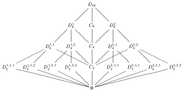
• Various types of rings and their relations:

Topics: Real Analysis

• Properties of Metric Spaces
• The Cauchy-Schwarz Inequality
• Definitions of Sequences and Series
• Testing Convergence of sequences and series
• Cauchy sequences and completeness
• Commuting limiting operations:
  • $[\frac{\partial}{\partial x}, \int dx]$
• Uniform and point-wise continuity
• Lipschitz Continuity

Big Theorems

• Completeness: Every Cauchy sequence in $\RR^n$ converges.
• Generalized Mean Value Theorem
  
  $$f,g\text{ differentiable on } [a,b] \implies \\ \exists c\in[a,b] : \left[f ( b ) - f ( a ) \right] g' ( c ) = \left[g ( b ) - g ( a )\right] f' ( c )$$
  • Take $g(x) = x$ to recover the usual MVT
• Bolzano-Weierstrass: every bounded sequence in $\RR^n$ has a convergent subsequence.
• Heine-Borel: in $\RR^n, X$ is compact $\iff X$ is closed and bounded.

Topics: Point-Set Topology

General Concepts

• Open/closed sets
• Connected, disconnected, totally disconnected, etc
• Mostly topics related to metric spaces

Useful Facts

• Topologies are closed under
  • Arbitrary unions:
    $$U_j \in \mathcal{T} \implies \union_{j\in J} U_i \in \mathcal{T}$$
  • Finite intersections:
    $$U_i \in \mathcal{T} \implies \intersect_{i=1}^n U_i \in \mathcal{T}$$
• In $\RR^n$, singletons are closed, and thus so are finite sets of points
  • Useful for constructing counterexamples to statements

Topics: Complex Analysis

General Concepts

• $n\dash$th roots:
  
  $$e^{\frac{ki}{2\pi n}}, \qquad k = 1, 2, \cdots n-1$$
• The Residue theorem:
  
  $$\oint_C f(z)~dz = 2\pi i \sum_k \mathrm{Res}(f, z_k)$$
  • Exams often include one complex integral
  • Need a number of other theorems for actually computing residues

Topics: Discrete Mathematics + Combinatorics

General Concepts

• Graphs, trees
• Recurrence relations
• Counting problems
  • e.g. number of nonisomorphic structures
• Inclusion-exclusion, etc

Example Problem 1

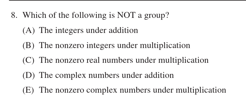
Example Problem 1

C, because $\ZZ-\theset{0}$ lacks inverses
(Would need to extend to $\QQ$)

Example Problem 2

Example Problem 2

So E, because the limit needs to be path-independent.

Example Problem 3

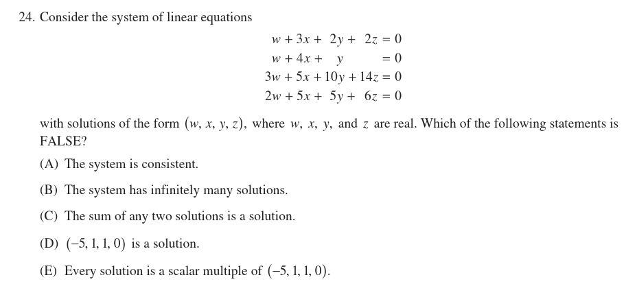
Example Problem 3

Don’t row-reduce or invert! Just one computation

Example Problem 3

So D, A are true. C is true because it’s a homogeneous system. B is true because $A\vector x = 0 \implies A (t\vector x) = tA\vector x = 0$ which means $t\vector x$ is a solution for every $t$. By process of elimination, E must be false.

Example Problem 4

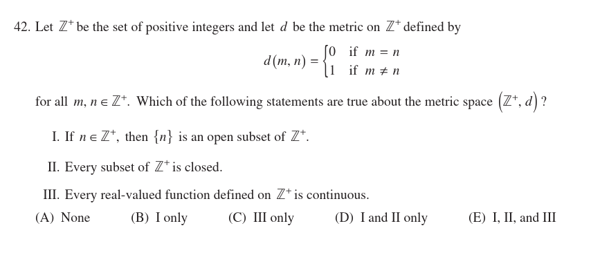
Example Problem 4

Note $N_{\frac{1}{2}}(x) = \theset{x}$, so every singleton is open. Any subset of $\ZZ$ is a countable union of its singletons, so every subset of $\ZZ$ is open. The complement any set is one such subset, so every subset is clopen. The inverse image of any subset of $\RR$ under any $f:\ZZ \to \RR$ is a subset of $\ZZ$, which is open, so every such $f$ is continuous. So E.